One million conductor elements in one minute, on a 16 GB laptop A short history of our solvers, and the published numbers behind the claim: what the established methods do on this problem, and what we had to change twice

A short history of our solvers, and the published numbers behind the claim: what the established methods do on this problem, and what we had to change twice

One million elements, one minute

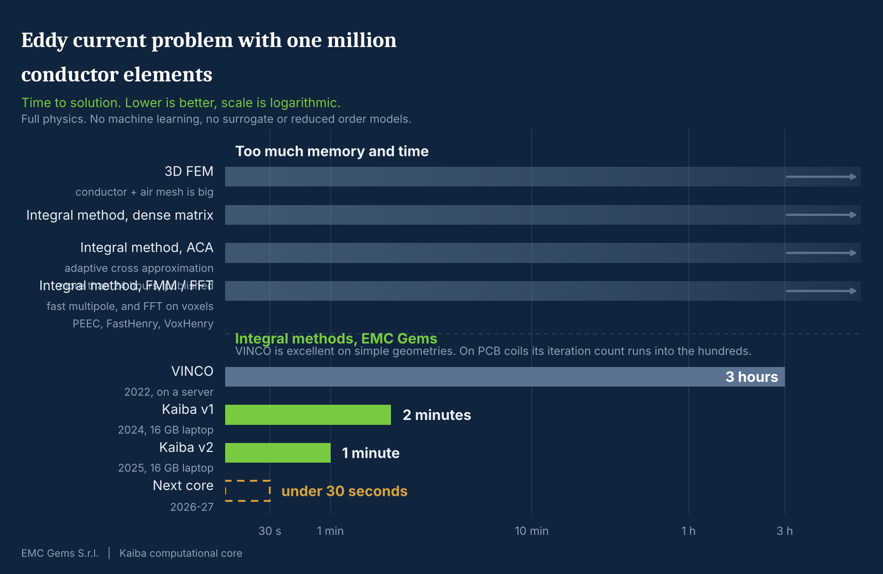
We solved an eddy current problem with one million conductor elements on a laptop with 16 GB of RAM, at 1 MHz, in about one minute, using about 4 GB.

One million elements is the copper only: every trace and every turn of wire. The surrounding air is never discretised, and the electromagnetic field in the surrounding space still comes out of the solution.

At 1 MHz the skin depth in copper is about 65 micrometres, roughly twice the 35 micrometres of 1 oz copper, so the current is already redistributing itself across the trace. The cost of the solution does not depend on the frequency over the whole range where the magnetoquasistatic approximation holds; above that you need a full wave model, and that is a limit of the physics, not of the solver.

zoom

Why the conventional routes struggle

Four established approaches are the obvious things to try. All four are good tools inside their range, and none of them gets to this result on this machine. The numbers below are published, and three of the four comparisons come from our own papers.

Finite elements

I have twenty years of experience with eddy current problems in finite elements, including writing the codes, so this is not an argument about anyone else's software. Three things keep the method out of this class of problem. The air has to be meshed too, and for a printed circuit board one million elements in the copper means ten to twenty million in the air, often more; in many real cases the air mesh around a multilayer coil with 35 micrometre copper simply cannot be built. Convergence: in the air the conductivity is zero, the term that makes the curl curl system non singular disappears, and what is left has a very large kernel of gradients. How badly this bites depends on formulation and preconditioner, and on air dominated geometries we have not found a combination, multigrid included, that converges in few iterations. Motion generally means rebuilding the mesh at every position, unless the motion has the symmetry a sliding interface can exploit, which covers a rotating machine and not a target that also tilts and shifts.

Integral methods, and what the name coversIntegra

l methods come in three forms: volume integral, surface integral and PEEC, the partial element equivalent circuit method. PEEC was originally built on parallelepipeds with current directions fixed in advance; give it finite element style basis functions and it becomes a volume integral method. What they share is the property that matters here: only the conductors are discretised, with no air mesh and no truncation boundary. What separates them is how they handle the dense matrix that this choice produces.

Dense matrices

The matrix is full, so memory grows with the square of the unknowns. On the million element benchmark of our CMAME paper the standard dense formulation allocates 8,141 GB, about eight terabytes. There is nothing to tune.

ACA, adaptive cross approximation

The standard answer in the literature, and it is worth being blunt about how little it buys. On a 252 thousand tetrahedra model, compression brought peak memory to 8 percent of the dense case, from 426 GB to 34.8 GB, but the total time only to 43 percent, from 26,495 seconds to 11,437. A factor of twelve on memory, a factor of two on time, in a problem where the gap to close is three orders of magnitude.At scale the gap becomes decisive. On the million element benchmark, on the same machine, ACA took more than 24 hours where the method described below took 649 seconds, and it still needed more memory for a quarter of the problem. Compression is what makes these models fit. It is not what makes them fast.

Fast multipole

The best of the published compression techniques in our own benchmark. The usual objection is the iteration count, but there is a second one that is almost never counted: the cost of a single interaction. With the usual element bases a pair of elements does not cost one integral but one per pair of basis functions, which is thirty six weighted interaction integrals for a six edge basis and sixteen for a face based Raviart Thomas or Rao Wilton Glisson basis. The VINCO framework uses element wise uniform basis functions, and a pair of tetrahedra costs one. That is not a trade of accuracy for speed. Our papers state the two as equivalent: the VINCO discretisation gives the same discrete solution, and on a tetrahedral mesh its stiffness matrix coincides with the one built from Raviart Thomas basis functions.To be exact, that factor is the cost of the direct, near field part of the operator, and fast multipole acceleration changes how the far field is evaluated. It does not remove the complexity that spatially varying basis functions introduce, but the remaining overhead is implementation dependent, so read sixteen or thirty six as a near field cost and not as a universal per iteration one.

FFT on voxels

Of everything above, this is the only route that is really competitive on feasibility. The comparison has to be made at equal accuracy, though, and that is where it comes apart. One million voxels is not one million tetrahedra.We have the numbers for a real case: the transmitter coil of an inductive position sensor, 35 micrometre copper on 0.8 mm board, measured on a Bode100 from 10 kHz to 10 MHz and simulated with all three approaches.

The FFT approach required a computational grid of approximately 120 million cells, at 35 micrometre resolution, whereas the geometry conforming formulation used about 800,000 conductor tetrahedra. The tetrahedral model also agreed more closely with the experimental measurements, precisely because it represents the curved features.There is a second cost buried in that grid. The FFT works on the whole box, not only on the cells that contain copper: in that example 229 thousand conductor cells sat inside a grid of 120 million, an air to conductor volume ratio of 522. The cost of the air comes back through the window, in the one family of methods that existed to avoid it.None of this is an objection invented for a blog post.

The CMAME paper names three limitations of the voxel route: the FFT buys its speed by requiring a Cartesian mesh; a voxelised geometry carries the well known staircase error, the same error that makes everyone prefer finite elements over finite differences; and a voxel grid rules out local mesh refinement. Our conclusion from that study, stated as we found it, is that voxel grids with FFT acceleration suit problems with fewer than about a million elements, with no curved features, and with a geometry well aligned to the structured grid. A coil on a printed circuit board is none of those three things.

zoom

From VINCO to Kaiba

VINCO was a breakthrough, and its numbers are public. A solid sphere of 1,030,656 tetrahedra: 649 seconds on a 32 core Threadripper with 256 GB, and the same problem in 1,220 seconds on a laptop with 16 GB of RAM, using 13.5 GB of peak memory. Ten to twenty iterations, consistently. It is patented together with the University of Udine, with the US patent granted, and its foundations are published in Computer Methods in Applied Mechanics and Engineering, one of the leading scientific journals in engineering simulation.

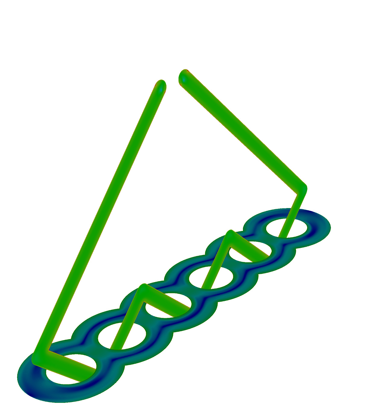
Then our own sensor geometries exposed its limits. The benchmarks in those papers are a sphere, a plate with a hole, a coil wound around a cylinder, and one printed circuit board coil of eight turns, 514,285 tetrahedra at 5 MHz, solved in 242 seconds. That last one is a single spiral in free space, and it is the easy end of our world. Add the second layer, the receive coils interleaved with the transmitter, and above all a conductive target a few tenths of a millimetre away across the airgap, and the iteration count climbs into the several hundreds.

Our estimate for the million element sensor benchmark with VINCO is about three hours

.Three hours is acceptable if you run one simulation. Our platforms run thousands inside an automatic optimisation loop, because that is how a high performance inductive sensor is actually designed: deform the receive coils, measure the linearity error, repeat. At three hours a run that loop does not exist. And a position sensor is the small end of what we want to reach: a DC-DC converter with its planes and shields, an electric machine with its real slot geometry, a wireless power pair with the metal around it, each a larger and harder model that deserves the same loop.We could have spent years tuning VINCO. Instead we went back to the mathematics and started again. The result is Kaiba, the first of a new class of solvers.It is worth being exact about the size of the two steps, because a chart with everything on one axis makes them look like rungs of the same ladder.

From PEEC to VINCO is a step inside one family: the same integral equation, the same kind of discretisation, a better factorisation of the matrix and a better way of applying it. It earned a patent and a paper, and it is continuous with what came before.

From VINCO to Kaiba is not that.

Measured in technology rather than in seconds, the distance from PEEC to VINCO is small compared with the distance from VINCO to Kaiba. It is also the one piece of our work we will never publish.On the sensor benchmark: about 8 GB and two minutes with Kaiba v1 in 2024, about 4 GB and one minute with Kaiba v2 in 2025, both on the same 16 GB laptop.

Why the scaling is the real result

The fair objection, which we would rather raise ourselves: one million conductor elements can probably be solved by one of the methods above on a workstation with 64 GB of RAM. Quite possibly true, and not the point.The point is what the same machine buys. At approximately 4 GB per million elements, memory is no longer the immediate bottleneck. We have verified linear scaling in both memory and computation time up to ten million elements, so a 64 GB workstation should take on the order of fifteen million. The fifteen is a short extrapolation beyond a measured ten: treat it as a projection and judge us on the ten.

At equal hardware, whether a laptop, a workstation or a cluster node, that reaches problem sizes the other routes do not reach at all. Entire inverter power stages with their planes and shields, complete motor windings with the real slot geometry, full sensor assemblies with the metal of the machine around them.

Those are not simulated today because no available tool returns an answer, not because nobody wants one.There is a quieter consequence too. A great deal of effort in this field goes into making a problem fit: coarsening the mesh, cutting the model along a symmetry plane that is not really there, homogenising a winding, dropping the shield. Those are accuracy decisions taken for memory reasons, and none of them appears in the final report.

What is next, and what is not in the box

There is no machine learning in this result. No surrogate, no reduced order model, no network trained on similar coils. Every number comes from solving Maxwell's equations for the geometry in front of it, which matters for a practical reason: a surrogate is accurate inside the space it was trained on and silently wrong outside it, and the designs worth simulating are the ones nobody has built yet.The step from VINCO to Kaiba was not profiling, vectorisation or a bigger machine, and neither was the step from two minutes to one. Each needed a change in the mathematics. The next change of that kind is already on paper and not yet in the code. Our bet is thirty seconds on the same laptop, and you can hold us to it.

Benchmark conditions and references

• Problem. Eddy current problem in the frequency domain, linear isotropic conductors in free space, skin and proximity effects resolved. 1,000,000 conductor elements, copper only, air not discretised. 1 MHz.

• Machine and result. Laptop with 16 GB of RAM, no cluster and no GPU. About one minute, setup and solve included, using about 4 GB with Kaiba v2 and about 8 GB with Kaiba v1.

• Scaling. Time and memory both linear in the number of conductor elements, verified up to ten million. Cost essentially independent of frequency within the magnetoquasistatic range.

• Earlier generation. VINCO, 2022, estimated at about three hours on this geometry class. Its published figures are for simpler benchmarks: 1,030,656 tetrahedra of a solid sphere in 1,220 seconds and 13.5 GB on the same class of laptop, 649 seconds on a 32 core server.

• Not used. Machine learning, surrogate models, model order reduction, symmetry reduction, geometric simplification.We publish the problems, the physics and the benchmark conditions. We do not publish the solver.

For the generation before Kaiba the record is public:

• M. Passarotto, S. Pitassi, R. Specogna, "Foundations of volume integral methods for eddy current problems", Computer Methods in Applied Mechanics and Engineering, vol. 392, 114626, 2022.

• A. Vacalebre, S. Pitassi, R. Specogna, "Low-rank compression techniques in integral methods for eddy currents problems", Computer Physics Communications, vol. 289, 108756, 2023.

• D. Voltolina, R. Torchio, P. Bettini, R. Specogna, P. Alotto, "Optimized cycle basis in volume integral formulations for large scale eddy-current problems", Computer Physics Communications, vol. 265, 108004, 2021.

Kaiba is the computational core inside both of our platforms: IPSMagic, which designs, optimises and validates inductive position sensors, and MAGMagic, which extracts the losses and parasitics of planar magnetics and power layouts. Both are licensed to major semiconductor and sensor manufacturers.

CALL TO ACTION

CTA heading: Try it on the problem that does not fit

CTA title: Bring us the geometry your current tool cannot meshIf you have a model your present tool cannot mesh, cannot fit in memory or cannot finish, that is the interesting case and we would like to see it.

Send us the geometry and the frequency range, and we will run it and show you the result, the conditions and the runtime.

If your existing flow handles it well, we will tell you that too.

Back to blog index